|
|
|
|
|
|
|
|
|
|
KAIST |
KAIST |
KAIST |
|
Ghent University |
KAIST |
|
|
|
|
|
|
|
|
|
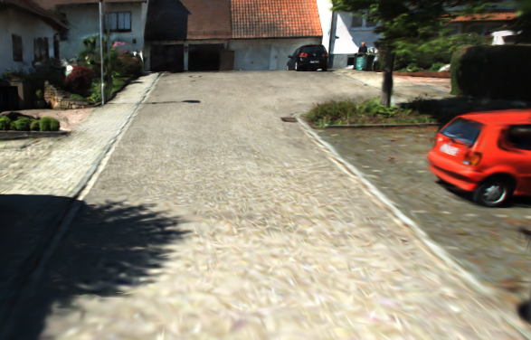
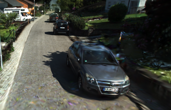
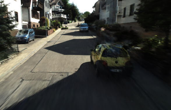
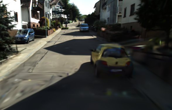
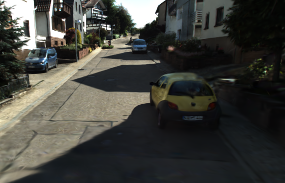
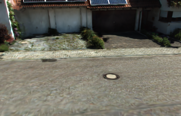
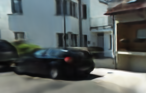
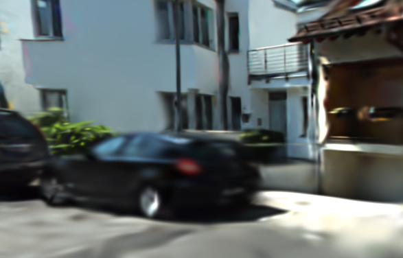
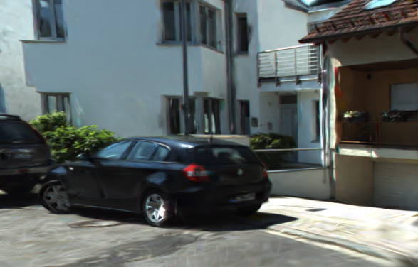
| Our method achieves high-fidelity renderings from views distanced from training camera distribution. |
|
|
|
|
|
|
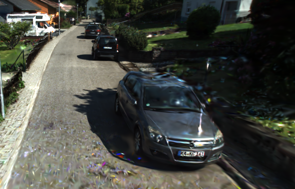
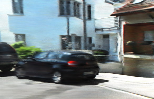
| Our method jointly reconstructs static scene with dynamic objects such as cars. |
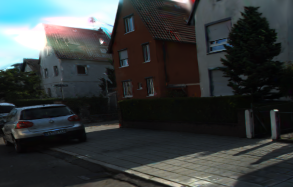
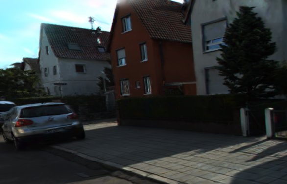
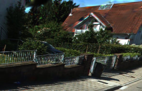
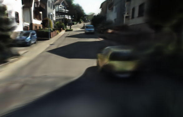
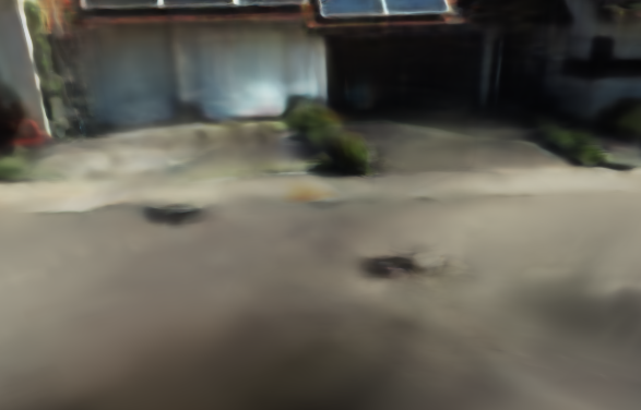
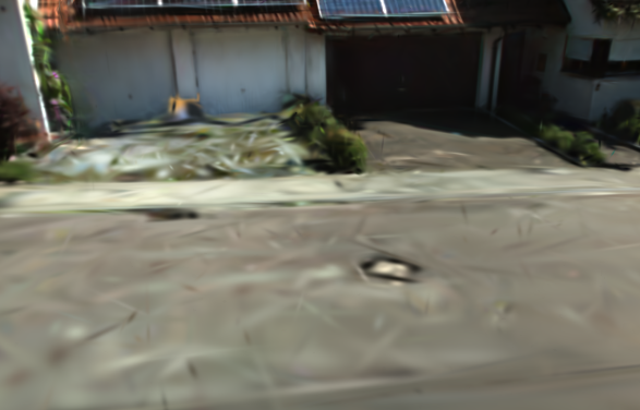
| We tackle the Extrapolated View Synthesis (EVS) problem on views such as looking left, right or downwards from train camera distributions. | |
|
|
|
 |
|
We initialize gaussian means using dense LiDAR map and point cloud from SfM.
We leveraged prior scene knowledge, such as surface normal estimation
and large-scale diffusion models, to improve rendering quality for EVS.
|
|
|
|
|
 |
The Lazy Covariance Optimization (LCO) Problem |
|
|
|
|
 |
|
Covariance Guidance Loss |
|
|
Our key idea is to guide the orientation and shape of covariances to make them behave like the
underlying scene surface. Specifically, we propose \(\mathcal{L}_{cov}\) =\(\mathcal{L}_{axis}\) + \(\mathcal{L}_{scale}\), where
\(\mathcal{L}_{axis}\) aligns covariance axes to a surface normal vector and
\(\mathcal{L}_{scale}\) minimizes the scale along the covariance axis aligned with surface normal
|
|
|
|
|
|
|
|
|
|
|
| Noise (score) predicted from a diffusion model \( \textbf{s}_{\theta} \) is proportional to the log-gradient of a prior distribution \( p(\textbf{x}) \), or \( \textbf{s}_{\theta}(\textbf{x}_{\tau}, \tau) \approx - \nabla_{\textbf{x}} \text{log} p(\textbf{x}) \). Thus, optimizing \( \textbf{x}_{\tau} \) to yield smaller score pushes \( \textbf{x} \) to our prior distribution \( p(\cdot) \). We model our prior distribution using Stable Diffusion fine-tuned with LoRA. |
|
|
|
|
|
|
|
|
|
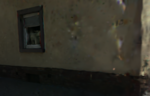
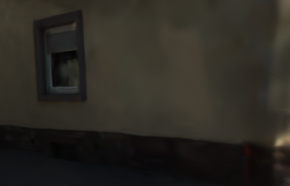
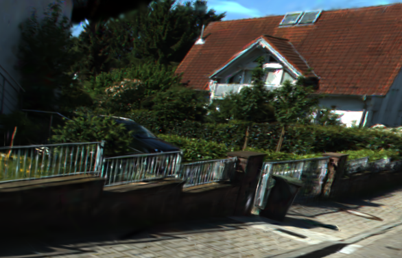
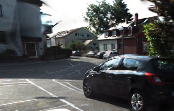
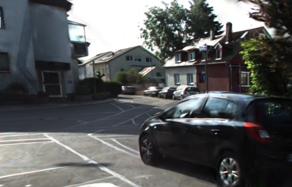
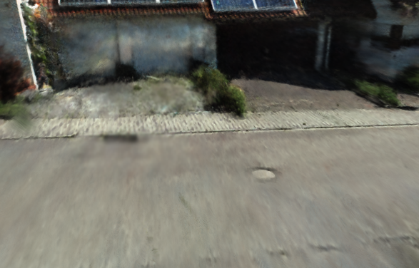
| EVS-D and EVS-LR refers to extrapolated views facing downwards and left/right, respectively. |
|
|
|
|
|
|
|
|
|
|
EVS-D
|
|
|
EVS-D
|
|
|
EVS-LR
|
|